
1. The morning I looked at the bill
On May 3rd, I ran a cost audit on Parjanya’s AWS account because the number I’d been carrying in my head — “it’s cheap, it’s a GPU worker and some Lambdas” — didn’t match what Billing was showing me.
It wasn’t cheap.
The account was running at roughly $100/day, and GPU EC2 accounted for most of that at the time: 57–65% of the bill. Two g4dn.2xlarge instances were running 24/7 on 100% on-demand capacity for our Qwen3-VL-8B image-quality worker.
Then I checked the launch template.
"OnDemandPercentageAboveBaseCapacity": 100A hundred percent.
The Terraform module already supported Spot allocation. The mixed_instances_policy had been there since March. I simply hadn’t enabled it.
That is where a typical cloud-cost story might end: find the waste, flip the switch, move on.
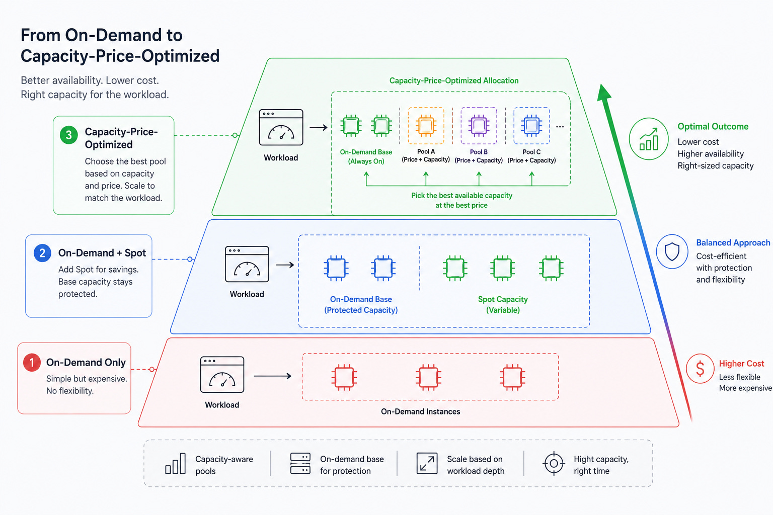
But that only answered one question:
Which pool should an instance come from?
It took me much longer to ask the second:
How many instances do I actually need?
That second question turned out to matter even more.
2. What I believed about Spot capacity — and what the data showed
I had an assumption I’d never re-tested: GPU Spot capacity in Mumbai wasn’t reliable enough to build around.
That assumption was the reason the ASG had remained on-demand-only since March. It wasn’t really an oversight. It was an old decision that I hadn’t revisited.
So before changing anything, I pulled seven days of Spot price history across the GPU instance types we could realistically use:
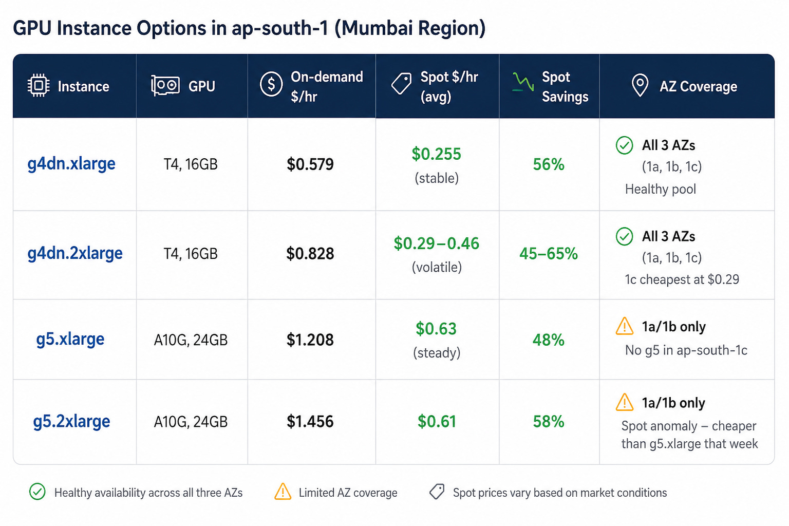
The assumption hadn’t been unreasonable when I made it. It was simply stale.
By May, g4dn.xlarge Spot capacity was looking healthy across all three availability zones. g5.xlarge was a different story: better GPU capacity, but available in only two AZs.
Rather than rely entirely on historical pricing, I ran a live canary.
I switched the ASG to Spot, terminated two on-demand instances, and sent the same workload through both configurations.
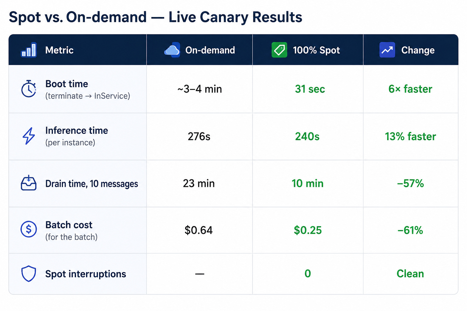
The measured result was a 61% reduction in cost per unit of work.
The important lesson wasn’t just about Spot.
The thing standing between me and that saving wasn’t a technical limitation. It was an assumption I had stopped questioning.
3. Why I didn’t go 100% Spot
Spot capacity can disappear with little warning.
Our worker also has a significant warm-up cost: pulling the container image and loading a roughly 17GB model. If an instance is reclaimed during warm-up, it produces no useful work.
So I didn’t want the entire fleet to depend on Spot availability.
The configuration became a combination of on-demand and Spot:
gpu_instance_types       = ["g5.xlarge", "g4dn.xlarge"]
on_demand_base_capacity  = 4
on_demand_percentage     = 0
spot_allocation_strategy = "price-capacity-optimized"
The idea is simple:
Keep a small on-demand base as insurance.
Use Spot for everything above that base.
Let the fleet scale with demand without paying the full on-demand price for every instance.
The on-demand base provides a floor that doesn’t depend on Spot availability. The Spot fleet provides most of the cost efficiency.
That combination turned out to be much more useful than thinking of Spot as an all-or-nothing decision.
4. Widening the pool — then narrowing it again
The next experiment was about the instance pool itself.
On July 9th, I saw several g4dn.xlarge Spot instances get reclaimed during warm-up. A pool containing only g5.xlarge and g4dn.xlarge was too narrow to absorb that pressure.
So I temporarily added:
g4dn.2xlargeg5.2xlarge
These instances had the same GPUs as their xlarge counterparts but more CPU and RAM than the workload really needed.
I wasn’t buying additional GPU throughput.
I was buying capacity insurance.
The idea was that price-capacity-optimized could use the larger instances only when the cheaper pools were under pressure. In that situation, paying a little more for an instance that actually becomes available can be better than waiting for a cheaper instance that doesn’t exist.
I calculated the worst-case premium before enabling it. Across a 12,000-image batch, the additional cost would have been roughly $3.
That was an acceptable temporary trade-off.
On July 28th, I removed the 2xlarge types again.
The reason was straightforward: as a permanent configuration, paying for extra CPU and RAM that the GPU workload didn’t use wasn’t attractive.
The temporary insurance had done its job. Once the capacity pressure eased, the simpler pool made more sense.
This also exposed an important operational principle:
A good configuration isn’t necessarily a permanent configuration.
Sometimes the right response to a capacity problem is to widen your options temporarily, then narrow them again when the underlying conditions change.
5. Two Spot capacity droughts
The experiments also exposed the limits of Spot.
July 9th
Mumbai’s g4dn Spot capacity went dry across the region.
The fleet dropped from five instances to one during a 450-image batch.
No allocation strategy could solve that. There simply wasn’t enough Spot capacity available.
The on-demand base was what kept the workload alive, so I increased the base from one to three instances that afternoon.
August 5th–7th
This time the problem was g5.xlarge.
There was no Spot support in one of its two available AZs, while the other experienced an on-demand capacity gap.
There were three launch failures over three days.
price-capacity-optimized was able to route around the problem by falling back to g4dn.xlarge, although the fallback introduced additional latency.
These two incidents changed how I think about Spot availability.
The answer isn’t simply that availability is “better” or “worse.”
It is better on average for some pools, but individual instance families can still experience significant capacity constraints.
Spot is a probability and capacity-management problem, not just a pricing problem.
6. What changed when I moved to price-capacity-optimized
There are two strategies that are easy to confuse:
capacity-optimized chooses the Spot pool with the deepest available capacity. Price isn’t part of the primary decision.
price-capacity-optimized considers both capacity availability and price, choosing among pools that have a reasonable likelihood of remaining available.
The distinction matters.
The May canary that produced the 61% cost reduction used capacity-optimized. I later moved to price-capacity-optimized on July 9th.
I don’t have a controlled, back-to-back experiment proving the exact dollar improvement from PCO. So I don’t want to manufacture one.
The decision was based on the allocation model and the observed capacity conditions rather than a clean A/B test.
That distinction matters when discussing infrastructure results:
Measured results and engineering judgments are not the same thing.
There was another useful discovery in the same change.
The Terraform module had an override issue that was silently alphabetizing the instance-type list rather than preserving the intended priority order.
So the configuration had effectively been saying one thing while the infrastructure was doing another.
It was a good reminder that infrastructure configuration needs the same level of testing and observability as application code.
7. The bigger question: how many instances?
This is where the more interesting problem appeared.
Until July 27th, both scale-up and scale-down used SimpleScaling.
The logic was effectively:
Is the queue empty?
If yes, scale down.
If no, scale up.
The problem is that this treats a queue containing 13 messages exactly like a queue containing 1,300 messages.
The system knew whether work existed.
It didn’t know how much work existed.
On July 27th, a small 13-image upload caused the fleet to scale to its maximum. Three of six instances processed nothing, and the timer-based scale-down took 69 minutes.
The post-incident calculation showed approximately 4.6 instance-hours spent for around 20 minutes of actual work.
The fix was to make scaling backlog-aware.
Instead of looking only at whether the queue was non-empty, the scaling logic now considers the combined backlog — visible and in-flight messages — and maps it to an explicit target fleet size:
backlog     target

1–25        → 1 instance
25–100      → 2
100–500     → 4
500+        → maximum
The policy also changed from incremental scaling to ExactCapacity.
Instead of saying:
Add one instance.
it says:
The fleet should contain four instances.
That difference is important.
Each scaling decision can converge directly on the desired fleet size rather than repeatedly increasing or decreasing the fleet one instance at a time.
In a later measured run, the same class of drain dropped from 69 minutes to 4 minutes.
But I made another mistake.
On August 8th, I reduced every scaling band by half.
That worked for small batches. It also meant that a 108-image production run on August 11th stayed on one instance for roughly 50 minutes when a second instance could have provided useful parallelism after its warm-up period.
Three days later, I adjusted the bands again rather than reverting the entire change.
The lesson was bigger than the individual thresholds:
Scaling needs to understand both price and workload depth.
Choosing the right Spot pool answers:
Which instance should I buy?
Autoscaling answers:
How many instances should I buy?
Those are different optimization problems.
And I had spent months tuning the first one before realizing the second one was costing me more.
8. Why this isn’t just a startup problem
It’s easy to think of backlog-blind scaling as an early-stage infrastructure problem.
I don’t think it is.
Any system where demand arrives in bursts can have the same problem.
Consider:
Batch customer onboarding
Large data imports
End-of-month reporting
Media processing
Scheduled analytics workloads
Seasonal traffic spikes
Any SaaS workload with uneven usage
A presence-based alarm can tell you:
There is work waiting.
It cannot tell you:
There are 20 messages versus 20,000 messages.
Those situations require completely different capacity decisions.
The mechanism is general:
Scaling decisions should consider the amount of work waiting, not just the existence of work.
The exact thresholds will vary by system, but the principle applies broadly.
9. What actually changed
Here are the results I can measure and reproduce:
61% lower cost per unit of work in the Spot vs. on-demand canary.
69 minutes → 4 minutes for a comparable production drain after moving to depth-aware ExactCapacity scaling.
~4.6 instance-hours consumed by an inefficient scaling response to a small workload.
~$3 maximum premium calculated for temporarily widening the Spot pool for a 12,000-image batch.
3 launch failures over 3 days during the August
g5.xlargecapacity issue.
The longer-term Cost Explorer data tells a similar story.
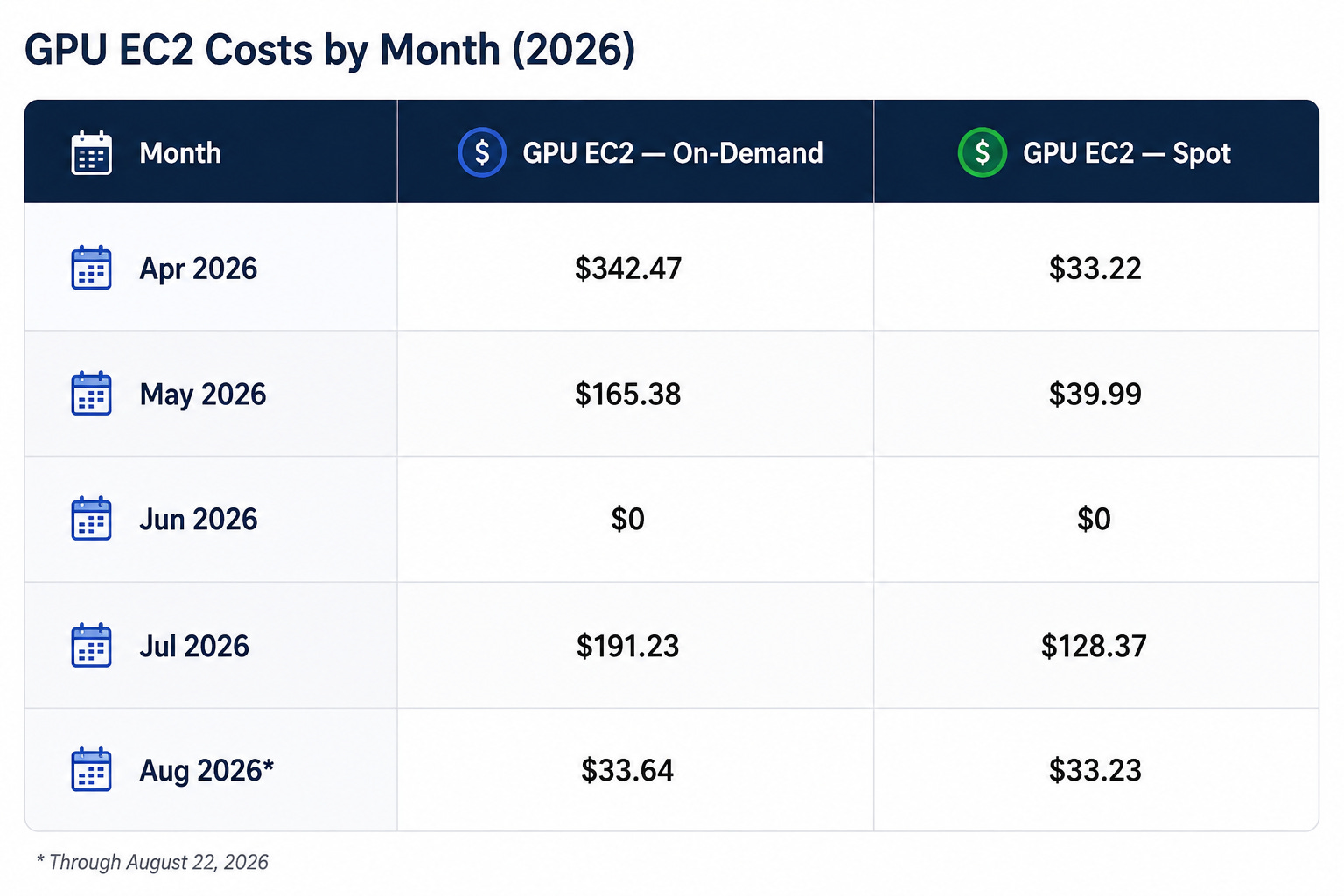
Across the GPU hours recorded this year, on-demand averaged roughly $0.64/hour, while Spot averaged roughly $0.30/hour — about a 53% discount.
For the 785 Spot hours recorded year-to-date, paying the blended on-demand rate would have cost approximately $505. Actual Spot spend was about $235.
That’s roughly $270 in measured savings from those Spot hours alone.
GPU EC2 has cost $967.85 year-to-date against $6,637.43 in total account spend through August 22 — roughly 15% of total spend.
The important point isn’t the exact percentage.
It is that the optimization moved from a simple:
“Can I get cheaper GPU instances?”
to a much broader question:
“Am I buying the right capacity, from the right pool, for the amount of work actually waiting?”
That is a much more useful infrastructure question.
10. The bigger takeaway: price and capacity must be optimized together
The biggest lesson from this exercise isn’t simply that Spot is cheaper than on-demand.
It is that price and capacity need to be considered together.
price-capacity-optimized matters because the cheapest Spot instance isn’t necessarily the cheapest option if that capacity isn’t available — or is likely to be reclaimed. A slightly more expensive pool with better capacity can be the better economic choice when the alternative is waiting for capacity that may never arrive.
That is the real value of price-capacity optimization:
Don’t optimize for the lowest price. Optimize for the lowest viable cost of reliable capacity.
The distinction became particularly clear during the capacity droughts I encountered. No allocation strategy can create capacity that doesn’t exist, which is why the on-demand base remained important. But when multiple Spot pools were available, price-capacity-optimized gave the fleet a better way to balance availability and cost instead of treating either one in isolation.
There is, however, a second layer that is just as important.
price-capacity-optimized answers:
Which capacity should I use?
Autoscaling answers:
How much capacity do I need?
Those are separate problems.
The configuration that ultimately worked for me brought both together:
Keep an on-demand base as protection against a complete Spot capacity shortage.
Use price-capacity-optimized Spot allocation to balance price and capacity across viable pools.
Keep multiple instance options available when capacity is constrained, but avoid permanently paying for resources the workload doesn’t actually use.
Scale based on backlog depth, rather than simply checking whether work exists.
Use ExactCapacity targets so the fleet converges directly on the capacity the workload needs.
This changed how I think about compute optimization.
The goal isn’t to find the cheapest instance.
It isn’t even to find the cheapest Spot pool.
The goal is to find the right amount of reliable capacity at the lowest practical cost.
That is what price-capacity-optimized ultimately taught me: price optimization without capacity awareness is incomplete, and capacity optimization without workload awareness can still waste money.
The real optimization happens when all three line up:
the right pool → the right price → the right amount of capacity.
11. The connection to context engineering
This is where this experiment connects with the earlier post on Context Engineering and Context Debt.
Context Engineering and Context Debt

TL;DR: I noticed Haiku 4.5 being spawned as a subagent during an Opus 4.7 session. That observation opened a data investigation that revealed ~77% of my token spend was context accumulation waste, not productive reasoning. This is the framework I built to fix it — and the problem has a name:
The two problems look different, but the underlying optimization pattern is surprisingly similar.
In context management, you have to decide:
Which information belongs in the context?
Then separately:
How much context should the model actually carry?
The GPU fleet has the same two layers.
Price-capacity-optimized answers:
Which pool should the instance come from?
Depth-aware scaling answers:
How many instances does the workload justify?
Getting the first decision right doesn’t automatically make the second one right.
That was the mistake I made.
I optimized the price and availability of each unit without first asking whether I needed that many units.
The same pattern appears in context management: a good retrieval strategy can still become expensive if the context budget itself isn’t being managed.
The broader lesson for me is simple:
Optimization is rarely one decision. It is usually a stack of decisions.
You can optimize the individual resource and still waste money because you’re using too much of it.
You can optimize the model and still waste tokens because you’re sending too much context.
You can optimize the database query and still waste resources because you’re running it too many times.
The useful question is therefore not just:
“What’s the cheapest way to do this?”
It is:
“What is the minimum amount of the right resource needed to do this reliably?”
That is the question I should have asked much earlier.
Configuration referenced in this post reflects the production setup as of August 12, 2026. Cost figures are based on a Cost Explorer pull covering January 1 through August 22, 2026.
