
Parjanya 2.0 — an AI-powered photography curation platform that combines CLIP-IQA for real-time scoring with Qwen3-VL-8B for deep visual understanding.
Today I would like to delve into the tooling story: how a single developer, working across five repositories, multiple AWS services, and a custom ML inference pipeline, managed to ship the entire VLM integration in under two weeks. I had been using various AI coding assistants for months. But this build was different. This was the first time I felt like I had a genuine engineering partner — one that could hold the full architecture in its head across multi-hour debugging sessions, reason about GPU memory layouts, and catch serialization bugs buried three abstraction layers deep.
This post is about what I learned using Claude Opus 4.6 with its 1M token context window for production ML infrastructure work. Not benchmarks. Not synthetic tests. Real observations from a real build, with real production failures at 2 AM.
The Build: What Is Being Built
Parjanya’s VLM pipeline is a SageMaker Batch Transform system that runs nightly inference on thousands of wildlife and nature photographs.
The model — Qwen3-VL-8B-Instruct — evaluates each image for quality, composition techniques (rule of thirds, leading lines, symmetry), and generates natural-language descriptions. The results feed back into DynamoDB and surface in a React frontend with a two-track pipeline visualization.
The infrastructure spans five repositories:
- **parjanya-ml** — Lambda handlers, SageMaker container, IQA engine, batch orchestration
- **parjanya-frontend** — React + Vite with VLM enrichment UI, pipeline status, score panels
- **parjanya-backend** — FastAPI with DynamoDB integration
- **parjanya-ops** — Terraform modules for IAM, networking, storage
- **parjanya-shared-libraries** — Python package with schemas and constants
Getting a custom Docker container with a quantized 8-billion parameter VLM running on SageMaker Batch Transform involved touching every single one of these repositories. The changes cascaded: the inference script needed GPU-aware dtype selection, the Dockerfile needed pinned dependency versions, the batch trigger Lambda needed DynamoDB Decimal serialization, the poller needed composition field propagation, the frontend needed new TypeScript interfaces, and the Terraform modules needed updated IAM policies.
This is the kind of cross-cutting work where context is everything.
The 1M Context Window: What It Actually Means in Practice
Let me be direct about something: I used ~10% of the 1M context window in any given session. That number sounds damning until you understand what it represents!
It Is Not About Filling the Window
The 1M context window is not a bucket you fill. It is a safety net that changes how you work. With a 128K or even 200K window, you are constantly managing context — summarizing, re-explaining, re-pasting code. You develop an anxiety about context loss. You start breaking problems into artificially small pieces not because the problem demands it, but because your tool demands it.
With 1M tokens, that anxiety disappears. And its absence changes your behaviour in ways I did not expect:
You stop pre-optimizing your prompts. Instead of carefully crafting minimal context windows, you just work. Paste the full Dockerfile. Include the entire inference script. Share the complete CloudWatch log dump. The model handles it.
Debugging sessions become continuous. Our VLM deployment failed eight times before succeeding. Each failure was a different root cause — OCI manifests, S3 permissions, Decimal serialization, instance quotas, transformers version drift, missing torchvision, BF16-on-T4 memory overflow, and finally, CPU offloading performance.
In a smaller context window, I would have lost the thread by failure three. With 1M, the model remembered every previous fix attempt and could reason about why this failure was different from the last.
Cross-repository reasoning becomes natural. When debugging why the batch trigger submitted zero images despite 4,942 records being in DynamoDB, the model held the Lambda handler code, the DynamoDB schema, the JSONL manifest format, and the CloudWatch error logs simultaneously. The root cause — Python’s `json.dumps` choking on DynamoDB’s `Decimal` type — was buried three abstraction layers deep. Finding it required connecting dots across files that no human would hold in working memory at once.
The Session Continuity Effect
Perhaps the most under appreciated aspect of 1M context is session continuity. When I hit the context limit after a particularly dense debugging session, the model generated a comprehensive session summary that captured not just what we had done, but the state of every in-flight problem. The next session picked up exactly where we left off — no re-explanation, no context rebuilding, no lost nuance.
This matters enormously for ML infrastructure work where debugging is inherently stateful. The GPU memory calculation that informed our quantization decision depended on understanding six previous failed deployments. Strip that history away, and you lose the reasoning chain.
Opus 4.6 for ML Infrastructure: Where It Excelled
GPU Memory Reasoning
The single most impressive moment in this build was the 4-bit quantization diagnosis. The VLM container was running — inference was succeeding — but each image took eight minutes instead of the expected thirty seconds. The CloudWatch logs showed a single warning line buried among hundreds of info messages:
WARNING Some parameters are on the meta device because they were offloaded to the cpu.
Opus immediately understood the implication chain: Qwen3-VL-8B in FP16 consumes approximately 16GB (8 billion parameters at 2 bytes each). The T4 GPU has exactly 16GB VRAM. That leaves zero headroom for the KV cache and attention buffers. Hugging Face’s `accelerate` library, configured with `device_map=”auto”`, silently offloads overflow layes to CPU. CPU inference is orders of magnitude slower. Therefore, the fix is not a timeout adjustment or a retry — it is a fundamental memory reduction via 4-bit NF4 quantization.
This was not a lookup. It was multi-step reasoning across hardware specifications, library behaviour, model architecture, and deployment configuration. The model then produced a complete `BitsAndBytesConfig` with parameter-by-parameter justification — why NF4 over FP4, why double quantization, why float16 compute dtype specifically for the T4’s lack of native BF16 support.
The result: 13x speedup. Eight minutes per image dropped to thirty-eight seconds. The entire batch cost projection went from an impractical $340 down to $27.
Dependency Chain Debugging
ML infrastructure has notoriously deep dependency chains. Our container failed five times before reaching the performance issue, each time for a completely different reason. Opus tracked the full history and used it productively:
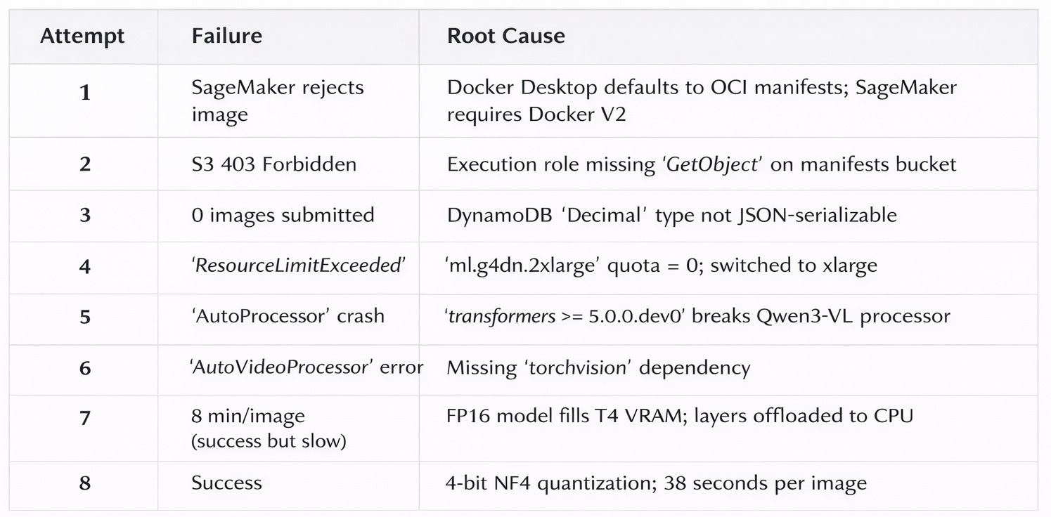
By attempt five, a smaller context model would have lost the thread of attempts one through four. Opus used the full failure history to eliminate hypotheses. When the `AutoProcessor` crashed, it did not suggest re-checking S3 permissions — it knew those were already fixed. It went straight to the `transformers` version as the novel variable.
Cross-Repository Code Generation
When we added composition analysis (detecting rule of thirds, leading lines, symmetry, etc.), the change touched four repositories simultaneously: the VLM inference prompt, the batch poller’s field propagation, the frontend TypeScript interfaces, and the React visualization components. Opus generated all four changes in a single coherent pass, with the field names aligned across Python, DynamoDB, and TypeScript — no mismatches, no forgotten fields.
The Model Tier Strategy: Opus, Sonnet, and Haiku
I did not use Opus exclusively. Over the course of the build, I developed an informal tiering strategy based on task complexity:
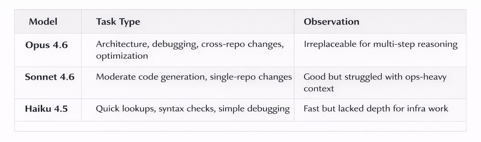
The critical observation: Sonnet 4.6, even with 1M context, was noticeably less effective for operations-heavy tasks like debugging SageMaker deployment failures or reasoning about GPU memory hierarchies. It would sometimes suggest re-trying the same approach that had already failed, or miss the implication of a warning message that Opus caught immediately. For pure code generation — writing a React component, implementing a Lambda handler — Sonnet was efficient. But for the diagnostic work that dominated this build, Opus was the difference between a one-hour fix and a one-day rabbit hole.
Haiku served a narrow but valuable role: quick validation checks. “Is this the right AWS CLI flag?” “What’s the torchvision version that matches torch 2.5.1?” For these atomic lookups, Haiku’s speed justified the quality tradeoff.
My rough allocation across the build: Opus handled about 80% of the work, Sonnet about 15% (mainly frontend component generation), and Haiku about 5% (quick checks during debugging). against originally planned in the month of January 2026
Claude Code vs. Cowork: A Solo Developer’s Perspective
I used both Claude Code (the CLI tool) and Cowork (the desktop agent) during this build. My experience as a solo developer working on poly-repo infrastructure was nuanced.
Where Cowork Felt Right
Visual task tracking. The todo list widget showing task progress was genuinely useful for multi-step deployments. When you are running through a seven-step build-push-deploy-submit cycle, visual confirmation of what is done and what is next reduces cognitive load.
File creation workflow. Generating documentation, cost spreadsheets, and configuration files felt natural in Cowork’s file-oriented interface. The ability to create and present files with download links was seamless.
Conversational debugging. Pasting CloudWatch logs, discussing error messages, iterating on solutions — the chat interface was more comfortable than a terminal for this back-and-forth.
Where It Hit Limits
Sandbox isolation. Cowork runs in a sandboxed environment. It cannot access local environment variables, AWS credentials, or push to GitHub directly. For infrastructure automation — where the whole point is interacting with external services — this creates friction. Every Docker push, every SageMaker API call, every git operation required copying commands to a terminal. The sandbox is a sensible security boundary, but for a solo developer doing infra work, it adds a context-switching tax.
No persistent shell state. Environment variables set in one Bash invocation do not persist to the next. For infrastructure work where you are building up state (`JOB_NAME`, `ACCOUNT_ID`, container digests), this means re-setting variables or passing them inline every time. Network restrictions. The sandbox cannot reach GitHub, AWS, or Docker registries directly. This is by design — security — but it means Cowork excels at reasoning and code generation while the developer handles execution. For pure software engineering (writing code, designing architectures), this split works. For DevOps/MLOps where execution is the work, it is more limiting.
The Verdict
For poly-repo infrastructure work as a solo developer, I would recommend Cowork for planning, code generation, documentation, and debugging analysis — then Claude Code or manual terminal work for execution. The combination leverages each tool’s strengths. Cowork’s 1M context and visual interface for the thinking; your terminal’s full system access for the doing.
Best Practices: Getting the Most from 1M Context
After this build, I have developed a set of practices specifically for leveraging large context windows in complex infrastructure projects:
1. Do Not Summarize Prematurely
The instinct from smaller-context models is to summarize aggressively. Resist it. When debugging a SageMaker deployment, the raw CloudWatch logs — all of them — are more valuable than a summary. The model can pattern-match across hundreds of log lines in ways that summaries destroy. I found that pasting full error outputs, complete Dockerfiles, and entire handler files produced dramatically better results than curated snippets.
2. Let Failures Accumulate in Context
Our eight-attempt deployment journey would have been impossible to navigate without the full failure history in context. Each failure informed the next diagnosis. When the model could see that attempts one through four had already ruled out permissions, serialization, and quota issues, it could focus attempt five on the novel variable (library version). This cumulative elimination process is the 1M window’s killer feature for debugging.
3. Work in Long Sessions for Complex Problems
Context windows reward sustained engagement. A two-hour debugging session where the model accumulates understanding of your infrastructure is far more productive than five separate twenty-minute sessions that each start cold. The model develops what I can only describe as situational awareness — it knows your AWS account structure, your naming conventions, your DynamoDB key schema, which fixes have already been applied. This accumulated context is irreplaceable.
4. Use the Full Poly-Repo Context
Do not silo your work by repository. When I shared both the Python inference script and the TypeScript frontend interface in the same session, the model generated perfectly aligned field names across languages. When I included the Terraform IAM policy alongside the SageMaker deployment script, it caught permission gaps before they became runtime errors. The 1M window exists precisely for this kind of cross-cutting visibility.
5. Document as You Go, Not After
With the full build context available, the model generates remarkably accurate documentation. Our optimization deep-dive — covering the problem statement, root cause analysis, solution, performance comparison, and the complete deployment journey — was generated from the live session context. Every number, every timing, every error message was drawn from actual CloudWatch logs still in the conversation. Waiting to document after the session would have lost this fidelity.
6. Match Model Tier to Task Complexity
Not every task needs Opus. Use Haiku for quick lookups, Sonnet for straightforward code generation, and reserve Opus for the hard problems: multi-step debugging, architecture decisions, cross-repository changes, and performance optimization. This is not just about cost — it is about matching the model’s reasoning depth to the problem’s reasoning requirements.
The Quantization Story: Why This Needed Opus
I want to close with the optimization that made the entire pipeline viable, because I genuinely doubt it would have happened — or at least, not this efficiently — without Opus 4.6’s reasoning capabilities.
The problem: our VLM batch inference was technically working but taking eight minutes per image. At that rate, processing 5,000 images would take 27 days and cost over $300. The pipeline was functionally useless.
A less capable model might have suggested increasing the instance size, adding more memory, or splitting the batch into smaller chunks. These are reasonable suggestions that would have been wrong and a bomb(costs). The T4 GPU had enough raw compute — the issue was memory layout, not compute capacity.
Opus identified the real problem from a single log line, traced the implication chain through PyTorch’s memory management, Hugging Face’s `accelerate` library, and the T4’s hardware capabilities, then prescribed a specific quantization configuration with four interdependent parameters — each chosen for a concrete technical reason tied to our specific GPU.
The result was not incremental. It was a 13x speedup that transformed the pipeline from impractical to production-ready. The batch now runs in roughly 52 hours for $27. That is the kind of optimization that comes from deep technical reasoning, not pattern matching.
Looking Forward
Parjanya 2.0’s VLM batch is currently processing its first successful run as I write this — 4,942 images, ticking along at 38 seconds each, zero errors. The composition analysis, the quality assessments, the natural-language descriptions are all flowing into DynamoDB, ready for the frontend to surface.
What strikes me most about this build is not any single technical achievement. It is the shift in how I worked. For the first time, the limiting factor in a complex infrastructure project was not context management, re-explanation, or lost thread. It was the actual engineering problems. And with 1M tokens of context, even those became more tractable than I expected.
The 1M context window does not make hard problems easy. It makes hard problems addressable by removing the artificial constraint of forgetting. In ML infrastructure work, where every failure builds on the last and every fix informs the next, that is the difference between shipping and stalling.
📚 Further Reading & References
🧠 Large Context Models & Reasoning
Anthropic — Claude System Card & Capabilities
https://www.anthropic.com/news/claude-3-familyLost in the Middle: How Language Models Use Long Contexts — Liu et al. (2023)
https://arxiv.org/abs/2307.03172RoPE (Rotary Position Embeddings)
https://arxiv.org/abs/2104.09864ALiBi: Train Short, Test Long
https://arxiv.org/abs/2108.12409
⚙️ Quantization & Efficient Inference
QLoRA: Efficient Finetuning of Quantized LLMs
https://arxiv.org/abs/2305.14314BitsAndBytes Documentation
https://github.com/TimDettmers/bitsandbytesHuggingFace Accelerate — Big Model Inference
https://huggingface.co/docs/accelerate/main/en/usage_guides/big_modelingAWQ (Activation-aware Weight Quantization)
https://arxiv.org/abs/2306.00978GPTQ: Accurate Post-Training Quantization
https://arxiv.org/abs/2210.17323
🖼️ Vision-Language Models (VLMs)
Qwen-VL Technical Report
https://arxiv.org/abs/2308.12966CLIP: Learning Transferable Visual Models — OpenAI
https://arxiv.org/abs/2103.00020BLIP-2: Bootstrapping Language-Image Pretraining
https://arxiv.org/abs/2301.12597
☁️ ML Infrastructure & SageMaker
AWS SageMaker Batch Transform
https://docs.aws.amazon.com/sagemaker/latest/dg/batch-transform.htmlAWS ML Pipelines — Prescriptive Guidance
https://docs.aws.amazon.com/prescriptive-guidance/latest/ml-ops-pipelines/welcome.htmlDocker Image Manifest V2 vs OCI
https://docs.docker.com/registry/spec/manifest-v2-2/DynamoDB Data Types & JSON Serialization
https://docs.aws.amazon.com/amazondynamodb/latest/developerguide/DataModel.html
🧩 Debugging Distributed & ML Systems
Designing Data-Intensive Applications — Martin Kleppmann https://dataintensive.net
Google SRE Book
https://sre.google/sre-book/table-of-contents/The Tail at Scale — Dean & Barroso
https://research.google/pubs/pub40801/
⚡ GPU Systems & Performance
NVIDIA T4 Architecture Overview
https://www.nvidia.com/en-us/data-center/tesla-t4/PyTorch CUDA Memory Management
https://pytorch.org/docs/stable/notes/cuda.html
🧪 Real-World Engineering Blogs
HuggingFace Blog
https://huggingface.co/blogAWS Machine Learning Blog
https://aws.amazon.com/blogs/machine-learning/BitsAndBytes / Tim Dettmers Work
https://timdettmers.com
If you're building ML infrastructure in production, these resources go far beyond benchmarks — they explain the failure modes, trade-offs, and system behaviors that actually determine whether your pipeline ships or stalls.
